
Demo project
Logistic regression demo code, 資料來源: LINK
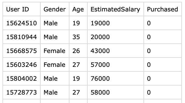
以下的 demo 是模擬如果我們透過對消費者的特性分析(年齡, 薪資)來預測消費者是否會真的購買商品. 此 demo 難度: 初階. 學習者可以嘗試用不同的模擬資料去訓練 AI 來做不同的目的.
import pandas as pd
import numpy as np
import matplotlib.pyplot as plt

# file from url as below
# https://www.kaggle.com/datasets/erscodingzone/user-datacsv/
dataset = pd.read_csv("User_Data.csv")

# input, 我們主要是看年齡 薪資 對 購買商品的 推算
# 用法 df.iloc[:, 2] # Selects the third column (index 2) for all rows
# df.iloc[1, 3] # Selects the element at the second row (index 1) and fourth column (index 3)
x = dataset.iloc[:, [2, 3]].values

# output, 買: 1 或是不買: 0
y = dataset.iloc[:, 4].values
# :, This colon indicates that you want to select all rows in the DataFrame.
# 4, This integer specifies that you want to select the column at index position 4.
# Remember that Python uses zero-based indexing, so the column at index 4 is actually
# the fifth column in your DataFrame.

# Splitting The Dataset: Train and Test dataset, 75% for training, 25% testing data
# 80% training, 20% validating data, 最推薦。這是最平衡的甜蜜點
# 70% training, 30% validating data, 訓練資料稍嫌不足,容易導致模型學不好
# 90% training, 10% validating data, 風險高。驗證集太小,評估結果不可信
from sklearn.model_selection import train_test_split

xtrain, xtest, ytrain, ytest = train_test_split(
    x, y, test_size=0.25, random_state=0)

from sklearn.preprocessing import StandardScaler

sc_x = StandardScaler()
xtrain = sc_x.fit_transform(xtrain)
xtest = sc_x.transform(xtest)
# scale the age variable value because the salary vs age, the number is too different
print(xtrain[0:10, :])

from sklearn.linear_model import LogisticRegression

#Train The Model
classifier = LogisticRegression(random_state = 0)
classifier.fit(xtrain, ytrain)

# After training the model, it is time to use it to do predictions on testing data.
y_pred = classifier.predict(xtest)

# Confusion Matrix
from sklearn.metrics import confusion_matrix

cm = confusion_matrix(ytest, y_pred)
print ("Confusion Matrix : \n", cm)

from sklearn.metrics import accuracy_score

print("Accuracy : ", accuracy_score(ytest, y_pred))

# Visualizing the performance of our model.
from matplotlib.colors import ListedColormap

X_set, y_set = xtest, ytest
X1, X2 = np.meshgrid(np.arange(start=X_set[:, 0].min() - 1,
                               stop=X_set[:, 0].max() + 1, step=0.01),
                     np.arange(start=X_set[:, 1].min() - 1,
                               stop=X_set[:, 1].max() + 1, step=0.01))

# 填滿的色塊
plt.contourf(X1, X2, classifier.predict(
    np.array([X1.ravel(), X2.ravel()]).T).reshape(
    X1.shape), alpha=0.75, cmap=ListedColormap(('red', 'green')))

plt.xlim(X1.min(), X1.max())
plt.ylim(X2.min(), X2.max())

#paint dots
for i, j in enumerate(np.unique(y_set)):
    plt.scatter(X_set[y_set == j, 0], X_set[y_set == j, 1],
                color=ListedColormap(('red', 'green'))(i), label=j)

plt.title('Classifier (Test set)')
plt.xlabel('Age')
plt.ylabel('Estimated Salary')
plt.legend()
plt.show()
User_Data.csv, 請到這邊下載 DOWNLOAD
以下為內容的參考資料
健康相關的 data 也可以拿來試試, 下載連結 DOWNLOAD
